


有句话叫“懂得了很多道理,依然过不好这一生。”用在这道题里很合适“懂得了每个过程的原理,依然写不好这代码。”
但抄完之后还是颇有收获的。
1、完成放射变换前向传播,f = wx + b
def affine_forward(x, w, b):
    """
    Computes the forward pass for an affine (fully-connected) layer.

    The input x has shape (N, d_1, ..., d_k) and contains a minibatch of N
    examples, where each example x[i] has shape (d_1, ..., d_k). We will
    reshape each input into a vector of dimension D = d_1 * ... * d_k, and
    then transform it to an output vector of dimension M.

    Inputs:
    - x: A numpy array containing input data, of shape (N, d_1, ..., d_k)
    - w: A numpy array of weights, of shape (D, M)
    - b: A numpy array of biases, of shape (M,)

    Returns a tuple of:
    - out: output, of shape (N, M)
    - cache: (x, w, b)
    """
    out = None
    ###########################################################################
    # TODO: Implement the affine forward pass. Store the result in out. You   #
    # will need to reshape the input into rows.                               #
    ###########################################################################
    reshaped_x = np.reshape(x,(x.shape[0],-1))
    #-1 是指剩余可填充的维度,所以这段代码意思就是保证reshape后的矩阵行数是N,剩余的维度信息都规则的排场一行即可。
    out = reshaped_x.dot(w) + b
    ###########################################################################
    #                             END OF YOUR CODE                            #
    ###########################################################################
    cache = (x, w, b)
    return out, cache
Testing affine_forward function:
difference: 9.769849468192957e-10
完成放射变换后向传播
def affine_backward(dout, cache):
    """
    Computes the backward pass for an affine layer.

    Inputs:
    - dout: Upstream derivative, of shape (N, M)
    - cache: Tuple of:
      - x: Input data, of shape (N, d_1, ... d_k)
      - w: Weights, of shape (D, M)
      - b: Biases, of shape (M,)

    Returns a tuple of:
    - dx: Gradient with respect to x, of shape (N, d1, ..., d_k)
    - dw: Gradient with respect to w, of shape (D, M)
    - db: Gradient with respect to b, of shape (M,)
    """
    x, w, b = cache
    dx, dw, db = None, None, None
    ###########################################################################
    # TODO: Implement the affine backward pass.                               #
    ###########################################################################
    reshaped_x = np.reshape(x,(x.shape[0],-1))
    dx = np.reshape(dout.dot(w.T),x.shape) #dout为上一层传播来的导数
    dw = (reshaped_x.T).dot(dout)
    db = np.sum(dout,axis = 0)
    #f = wx + b,则df/dx = w,df/fw = x,df/db = 1 再转为矩阵形式
    ###########################################################################
    #                             END OF YOUR CODE                            #
    ###########################################################################
    return dx, dw, db
Testing affine_backward function:
dx error: 5.399100368651805e-11
dw error: 9.904211865398145e-11
db error: 2.4122867568119087e-11
完成使用relu的前向传播
def relu_forward(x):
    """
    Computes the forward pass for a layer of rectified linear units (ReLUs).

    Input:
    - x: Inputs, of any shape

    Returns a tuple of:
    - out: Output, of the same shape as x
    - cache: x
    """
    out = None
    ###########################################################################
    # TODO: Implement the ReLU forward pass.                                  #
    ###########################################################################
    out = np.maximum(0,x)
    ###########################################################################
    #                             END OF YOUR CODE                            #
    ###########################################################################
    cache = x
    return out, cache
Testing relu_forward function:
difference: 4.999999798022158e-08
完成使用relu的后向传播
def relu_backward(dout, cache):
    """
    Computes the backward pass for a layer of rectified linear units (ReLUs).

    Input:
    - dout: Upstream derivatives, of any shape
    - cache: Input x, of same shape as dout

    Returns:
    - dx: Gradient with respect to x
    """
    dx, x = None, cache
    ###########################################################################
    # TODO: Implement the ReLU backward pass.                                 #
    ###########################################################################
    dx = (x>0) * dout
    #与所有x中元素为正的位置处,位置对应于dout矩阵的元素保留,其他都取0
    ###########################################################################
    #                             END OF YOUR CODE                            #
    ###########################################################################
    return dx
Testing relu_backward function:
dx error: 3.2756349136310288e-12
"三明治"模型:
def affine_relu_forward(x, w, b):
    """
    Convenience layer that perorms an affine transform followed by a ReLU

    Inputs:
    - x: Input to the affine layer
    - w, b: Weights for the affine layer

    Returns a tuple of:
    - out: Output from the ReLU
    - cache: Object to give to the backward pass
    """
    a, fc_cache = affine_forward(x, w, b) #线性模型
    out, relu_cache = relu_forward(a)  #激活函数
    cache = (fc_cache, relu_cache)   #(x,w,b,(a))
    return out, cache


def affine_relu_backward(dout, cache):
    """
    Backward pass for the affine-relu convenience layer
    """
    fc_cache, relu_cache = cache # fc_cache = (x,w,b) relu_cache = a
    da = relu_backward(dout, relu_cache)  #da = (x>0) * relu_cache
    dx, dw, db = affine_backward(da, fc_cache)
    return dx, dw, db
Testing affine_relu_forward and affine_relu_backward:
dx error: 2.299579177309368e-11
dw error: 8.162011105764925e-11
db error: 7.826724021458994e-12
loss层:
def svm_loss(x, y):
    """
    Computes the loss and gradient using for multiclass SVM classification.

    Inputs:
    - x: Input data, of shape (N, C) where x[i, j] is the score for the jth
      class for the ith input.
    - y: Vector of labels, of shape (N,) where y[i] is the label for x[i] and
      0 <= y[i] < C

    Returns a tuple of:
    - loss: Scalar giving the loss
    - dx: Gradient of the loss with respect to x
    """
    N = x.shape[0]
    correct_class_scores = x[np.arange(N), y] #得到正确的标签
    margins = np.maximum(0, x - correct_class_scores[:, np.newaxis] + 1.0) #delta = 1
    margins[np.arange(N), y] = 0 #跳过同类的那个
    loss = np.sum(margins) / N
    num_pos = np.sum(margins > 0, axis=1)
    dx = np.zeros_like(x)
    dx[margins > 0] = 1
    #大于0的才用求导数
    dx[np.arange(N), y] -= num_pos
    #对于正确标签那一类的梯度计算不同于其它类
    dx /= N
    return loss, dx


def softmax_loss(x, y):
    """
    Computes the loss and gradient for softmax classification.

    Inputs:
    - x: Input data, of shape (N, C) where x[i, j] is the score for the jth
      class for the ith input.
    - y: Vector of labels, of shape (N,) where y[i] is the label for x[i] and
      0 <= y[i] < C

    Returns a tuple of:
    - loss: Scalar giving the loss
    - dx: Gradient of the loss with respect to x
    """
    shifted_logits = x - np.max(x, axis=1, keepdims=True) #将每行中的数值进行平移,使得最大值为0
    Z = np.sum(np.exp(shifted_logits), axis=1, keepdims=True)
    log_probs = shifted_logits - np.log(Z)
    probs = np.exp(log_probs)
    N = x.shape[0]
    loss = -np.sum(log_probs[np.arange(N), y]) / N
    dx = probs.copy()
    dx[np.arange(N), y] -= 1
    #令其中每张样本图片(每行)对应于正确标签的得分都减一,再配以系数1/N之后,就得到了损失函数关于输入矩阵z的“梯度矩阵” dz

    #在例子中,对probs矩阵确切的切片含义是 probs[np.array([0, 1 ,2]), np.array([2, 0, 1])]
    #这就像是定义了经纬度一样,指定了确切的行列数,要求切片出相应的数值。对于上面的例子而已,就是说取出第0行、第2列的值;取出第1行、第0列的值;取出第2  行、第1列的值。于是,就得到了例子中的红色得分数值。切行数时,np.arange(N) 相当于是说“我每行都要切一下哦~”,而切列数时,y 向量(array)所存的数值型分类标签(0~9),刚好可以对应于probs矩阵每列的index(0~9),如果 y = np.array(['cat', 'dog', 'ship']) ,显然代码还这么写就会出问题了。
    dx /= N
    return loss, dx
Testing svm_loss:
loss: 8.999602749096233
dx error: 1.4021566006651672e-09
Testing softmax_loss:
loss: 2.302545844500738
dx error: 9.384673161989355e-09
两层的网络:
class TwoLayerNet(object):
    """
    A two-layer fully-connected neural network with ReLU nonlinearity and
    softmax loss that uses a modular layer design. We assume an input dimension
    of D, a hidden dimension of H, and perform classification over C classes.

    The architecure should be affine - relu - affine - softmax.

    Note that this class does not implement gradient descent; instead, it
    will interact with a separate Solver object that is responsible for running
    optimization.

    The learnable parameters of the model are stored in the dictionary
    self.params that maps parameter names to numpy arrays.
    """

    def __init__(self, input_dim=3*32*32, hidden_dim=100, num_classes=10,
                 weight_scale=1e-3, reg=0.0): ## weight_scale:初始化参数的权重尺度(标准偏差)
        """
        Initialize a new network.

        Inputs:
        - input_dim: An integer giving the size of the input
        - hidden_dim: An integer giving the size of the hidden layer
        - num_classes: An integer giving the number of classes to classify
        - weight_scale: Scalar giving the standard deviation for random
          initialization of the weights.
        - reg: Scalar giving L2 regularization strength.
        """
        self.params = {}
        self.reg = reg

        ############################################################################
        # TODO: Initialize the weights and biases of the two-layer net. Weights    #
        # should be initialized from a Gaussian centered at 0.0 with               #
        # standard deviation equal to weight_scale, and biases should be           #
        # initialized to zero. All weights and biases should be stored in the      #
        # dictionary self.params, with first layer weights                         #
        # and biases using the keys 'W1' and 'b1' and second layer                 #
        # weights and biases using the keys 'W2' and 'b2'.                         #
        ############################################################################
        # randn函数是基于零均值和标准差的一个高斯分布
        self.params['W1'] = weight_scale * np.random.randn(input_dim,hidden_dim) #(3072,100)
        self.params['b1'] = np.zeros((hidden_dim,)) #100
        self.params['W2'] = weight_scale * np.random.randn(hidden_dim,num_classes) #(100,10)
        self.params['b2'] = np.zeros((num_classes,)) #10
        ############################################################################
        #                             END OF YOUR CODE                             #
        ############################################################################


    def loss(self, X, y=None):
        """
        Compute loss and gradient for a minibatch of data.

        Inputs:
        - X: Array of input data of shape (N, d_1, ..., d_k)
        - y: Array of labels, of shape (N,). y[i] gives the label for X[i].

        Returns:
        If y is None, then run a test-time forward pass of the model and return:
        - scores: Array of shape (N, C) giving classification scores, where
          scores[i, c] is the classification score for X[i] and class c.

        If y is not None, then run a training-time forward and backward pass and
        return a tuple of:
        - loss: Scalar value giving the loss
        - grads: Dictionary with the same keys as self.params, mapping parameter
          names to gradients of the loss with respect to those parameters.
        """
        scores = None
        ############################################################################
        # TODO: Implement the forward pass for the two-layer net, computing the    #
        # class scores for X and storing them in the scores variable.              #
        ############################################################################
        #前向传播
        h1_out,h1_cache = affine_relu_forward(X,self.params['W1'],self.params['b1'])
        scores,out_cache = affine_forward(h1_out,self.params['W2'],self.params['b2'])
        ############################################################################
        #                             END OF YOUR CODE                             #
        ############################################################################

        # If y is None then we are in test mode so just return scores
        if y is None:
            return scores

        loss, grads = 0, {}
        ############################################################################
        # TODO: Implement the backward pass for the two-layer net. Store the loss  #
        # in the loss variable and gradients in the grads dictionary. Compute data #
        # loss using softmax, and make sure that grads[k] holds the gradients for  #
        # self.params[k]. Don't forget to add L2 regularization!                   #
        #                                                                          #
        # NOTE: To ensure that your implementation matches ours and you pass the   #
        # automated tests, make sure that your L2 regularization includes a factor #
        # of 0.5 to simplify the expression for the gradient.                      #
        ############################################################################
        #后向传播,计算loss和梯度
        loss,dout = softmax_loss(scores,y)
        dout,dw2,db2 = affine_backward(dout,out_cache)
        loss += 0.5 * self.reg * (np.sum(self.params['W1'] ** 2) + np.sum(self.params['W2'] ** 2))
        _,dw1,db1 = affine_relu_backward(dout,h1_cache)
        dw1 += self.reg * self.params['W1']
        dw2 += self.reg * self.params['W2']
        grads['W1'],grads['b1'] = dw1,db1
        grads['W2'],grads['b2'] = dw2,db2
        ############################################################################
        #                             END OF YOUR CODE                             #
        ############################################################################

        return loss, grads
Testing initialization ...
Testing test-time forward pass ...
Testing training loss (no regularization)
Running numeric gradient check with reg = 0.0
W1 relative error: 1.83e-08
W2 relative error: 3.12e-10
b1 relative error: 9.83e-09
b2 relative error: 4.33e-10
Running numeric gradient check with reg = 0.7
W1 relative error: 2.53e-07
W2 relative error: 2.85e-08
b1 relative error: 1.56e-08
b2 relative error: 7.76e-10
使用solver来验证
from __future__ import print_function, division
from future import standard_library
standard_library.install_aliases()
from builtins import range
from builtins import object
import os
import pickle as pickle

import numpy as np

from cs231n import optim


class Solver(object):
     """
     我们定义的这个Solver类将会根据我们的神经网络模型框架——FullyConnectedNet()类,
     在数据源的训练集部分和验证集部分中,训练我们的模型,并且通过周期性的检查准确率的方式,
     以避免过拟合。

     在这个类中,包括__init__(),共定义5个函数,其中只有train()函数是最重要的。调用
     它后,会自动启动神经网络模型优化程序。

     训练结束后,经过更新在验证集上优化后的模型参数会保存在model.params中。此外,损失值的
     历史训练信息会保存在solver.loss_history中,还有solver.train_acc_history和
     solver.val_acc_history中会分别保存训练集和验证集在每一次epoch时的模型准确率。
     ===============================
     下面是给出一个Solver类使用的实例:
     data = {
         'X_train': # training data
         'y_train': # training labels
         'X_val': # validation data
     '   y_val': # validation labels
         }   # 以字典的形式存入训练集和验证集的数据和标签
     model = FullyConnectedNet(hidden_size=100, reg=10) # 我们的神经网络模型
     solver = Solver(model, data,            # 模型/数据
                   update_rule='sgd',        # 优化算法
                   optim_config={            # 该优化算法的参数
                     'learning_rate': 1e-3,  # 学习率
                   },
                   lr_decay=0.95,            # 学习率的衰减速率
                   num_epochs=10,            # 训练模型的遍数
                   batch_size=100,           # 每次丢入模型训练的图片数目
                   print_every=100)
     solver.train()
     ===============================
     # 神经网络模型中必须要有两个函数方法:模型参数model.params和损失函数model.loss(X, y)
     A Solver works on a model object that must conform to the following API:
     - model.params must be a dictionary mapping string parameter names to numpy
         arrays containing parameter values. #
     - model.loss(X, y) must be a function that computes training-time loss and
         gradients, and test-time classification scores, with the following inputs
         and outputs:
     Inputs:     # 全局的输入变量
     - X: Array giving a minibatch of input data of shape (N, d_1, ..., d_k)
     - y: Array of labels, of shape (N,) giving labels for X where y[i] is the
       label for X[i].
     Returns:    # 全局的输出变量
     # 用标签y的存在与否标记训练mode还是测试mode
     If y is None, run a test-time forward pass and return: #
     - scores: Array of shape (N, C) giving classification scores for X where
       scores[i, c] gives the score of class c for X[i].
     If y is not None, run a training time forward and backward pass and return
     a tuple of:
     - loss: Scalar giving the loss  # 损失函数值
     - grads: Dictionary with the same keys as self.params mapping parameter
       names to gradients of the loss with respect to those parameters.# 模型梯度
     """

    def __init__(self, model, data, **kwargs):
        """
        Construct a new Solver instance.

        Required arguments:
        - model: A model object conforming to the API described above
        - data: A dictionary of training and validation data containing:
          'X_train': Array, shape (N_train, d_1, ..., d_k) of training images
          'X_val': Array, shape (N_val, d_1, ..., d_k) of validation images
          'y_train': Array, shape (N_train,) of labels for training images
          'y_val': Array, shape (N_val,) of labels for validation images

        Optional arguments:
        - update_rule: 优化算法,默认为SGD.
        - optim_config: 设置优化算法的超参数
        - lr_decay: 学习率在每个epoch的衰减率
        - batch_size: batch的大小
        - num_epochs: 在训练时,神经网络一次训练的遍数
        - verbose: 是否打印中间过程
        - num_train_samples: Number of training samples used to check training
          accuracy; default is 1000; set to None to use entire training set.
        - num_val_samples: Number of validation samples to use to check val
          accuracy; default is None, which uses the entire validation set.
        - checkpoint_name: If not None, then save model checkpoints here every
          epoch.
        """
        self.model = model
        self.X_train = data['X_train']
        self.y_train = data['y_train']
        self.X_val = data['X_val']
        self.y_val = data['y_val']

        # Unpack keyword arguments
        self.update_rule = kwargs.pop('update_rule', 'sgd')
        self.optim_config = kwargs.pop('optim_config', {})
        self.lr_decay = kwargs.pop('lr_decay', 1.0)
        self.batch_size = kwargs.pop('batch_size', 100)
        self.num_epochs = kwargs.pop('num_epochs', 10)
        self.num_train_samples = kwargs.pop('num_train_samples', 1000)
        self.num_val_samples = kwargs.pop('num_val_samples', None)

        self.checkpoint_name = kwargs.pop('checkpoint_name', None)
        self.print_every = kwargs.pop('print_every', 10)
        self.verbose = kwargs.pop('verbose', True)

        # Throw an error if there are extra keyword arguments 处理异常
        if len(kwargs) > 0:
            extra = ', '.join('"%s"' % k for k in list(kwargs.keys()))
            raise ValueError('Unrecognized arguments %s' % extra)

        # Make sure the update rule exists, then replace the string
        # name with the actual function
        if not hasattr(optim, self.update_rule):
            raise ValueError('Invalid update_rule "%s"' % self.update_rule)
        self.update_rule = getattr(optim, self.update_rule)

        self._reset()

   # 定义我们的 _reset() 函数,其仅在类初始化函数 __init__() 中调用
    def _reset(self):
        """
        Set up some book-keeping variables for optimization. Don't call this
        manually.
        """
        # Set up some variables for book-keeping
        self.epoch = 0
        self.best_val_acc = 0
        self.best_params = {}
        self.loss_history = []
        self.train_acc_history = []
        self.val_acc_history = []

        # Make a deep copy of the optim_config for each parameter
        self.optim_configs = {}
        for p in self.model.params:
            d = {k: v for k, v in self.optim_config.items()}
            self.optim_configs[p] = d


    def _step(self):
        """
        训练模式下,样本图片数据的一次正向和反向传播,并且更新模型参数一次。
        """
        # Make a minibatch of training data
        num_train = self.X_train.shape[0]
        batch_mask = np.random.choice(num_train, self.batch_size)
        X_batch = self.X_train[batch_mask]
        y_batch = self.y_train[batch_mask]

        # Compute loss and gradient
        loss, grads = self.model.loss(X_batch, y_batch)
        self.loss_history.append(loss)

        # Perform a parameter update
        for p, w in self.model.params.items():
            dw = grads[p]
            config = self.optim_configs[p]
            next_w, next_config = self.update_rule(w, dw, config)
            self.model.params[p] = next_w
            self.optim_configs[p] = next_config

    #保存checkpoint
    def _save_checkpoint(self):
        if self.checkpoint_name is None: return
        checkpoint = {
          'model': self.model,
          'update_rule': self.update_rule,
          'lr_decay': self.lr_decay,
          'optim_config': self.optim_config,
          'batch_size': self.batch_size,
          'num_train_samples': self.num_train_samples,
          'num_val_samples': self.num_val_samples,
          'epoch': self.epoch,
          'loss_history': self.loss_history,
          'train_acc_history': self.train_acc_history,
          'val_acc_history': self.val_acc_history,
        }
        filename = '%s_epoch_%d.pkl' % (self.checkpoint_name, self.epoch)
        if self.verbose:
            print('Saving checkpoint to "%s"' % filename)
        with open(filename, 'wb') as f:
            pickle.dump(checkpoint, f)

    #定义我们的 check_accuracy() 函数,其仅在 train() 函数中调用
    def check_accuracy(self, X, y, num_samples=None, batch_size=100):
        """
        Check accuracy of the model on the provided data.

        Inputs:
        - X: Array of data, of shape (N, d_1, ..., d_k)
        - y: Array of labels, of shape (N,)
        - num_samples: If not None, subsample the data and only test the model
          on num_samples datapoints.
        - batch_size: Split X and y into batches of this size to avoid using
          too much memory.

        Returns:
        - acc: Scalar giving the fraction of instances that were correctly
          classified by the model.
        """

        # Maybe subsample the data
        N = X.shape[0]
        if num_samples is not None and N > num_samples:
            mask = np.random.choice(N, num_samples)
            N = num_samples
            X = X[mask]
            y = y[mask]

        # Compute predictions in batches
        num_batches = N // batch_size
        if N % batch_size != 0:
            num_batches += 1
        y_pred = []
        for i in range(num_batches):
            start = i * batch_size
            end = (i + 1) * batch_size
            scores = self.model.loss(X[start:end])
            y_pred.append(np.argmax(scores, axis=1))
        y_pred = np.hstack(y_pred)
        acc = np.mean(y_pred == y)

        return acc


    def train(self):
        """
        Run optimization to train the model.
        """
        num_train = self.X_train.shape[0]
        iterations_per_epoch = max(num_train // self.batch_size, 1)
        num_iterations = self.num_epochs * iterations_per_epoch

        for t in range(num_iterations):
            self._step()

            # Maybe print training loss
            if self.verbose and t % self.print_every == 0:
                print('(Iteration %d / %d) loss: %f' % (
                       t + 1, num_iterations, self.loss_history[-1]))

            # At the end of every epoch, increment the epoch counter and decay
            # the learning rate.
            epoch_end = (t + 1) % iterations_per_epoch == 0
            if epoch_end:
                self.epoch += 1
                for k in self.optim_configs:
                    self.optim_configs[k]['learning_rate'] *= self.lr_decay #学习率衰减

            # Check train and val accuracy on the first iteration, the last
            # iteration, and at the end of each epoch.
            first_it = (t == 0)
            last_it = (t == num_iterations - 1)
            if first_it or last_it or epoch_end:
                train_acc = self.check_accuracy(self.X_train, self.y_train,
                    num_samples=self.num_train_samples)
                val_acc = self.check_accuracy(self.X_val, self.y_val,
                    num_samples=self.num_val_samples)
                self.train_acc_history.append(train_acc)
                self.val_acc_history.append(val_acc)
                self._save_checkpoint()

                if self.verbose:
                    print('(Epoch %d / %d) train acc: %f; val_acc: %f' % (
                           self.epoch, self.num_epochs, train_acc, val_acc))

                # Keep track of the best model
                if val_acc > self.best_val_acc:
                    self.best_val_acc = val_acc
                    self.best_params = {}
                    for k, v in self.model.params.items():
                        self.best_params[k] = v.copy()

        # At the end of training swap the best params into the model
        self.model.params = self.best_params
验证准确率:
model = TwoLayerNet()
solver = None

##############################################################################
# TODO: Use a Solver instance to train a TwoLayerNet that achieves at least  #
# 50% accuracy on the validation set.                                        #
##############################################################################
solver = Solver(model, data,
                  update_rule='sgd',
                  optim_config={
                    'learning_rate': 1e-3,
                  },
                  lr_decay=0.95,
                  num_epochs=10, batch_size=128,
                  print_every=100)
solver.train()
solver.best_val_acc
##############################################################################
#                             END OF YOUR CODE                               #
##############################################################################
(Iteration 1 / 3820) loss: 2.302693
(Epoch 0 / 10) train acc: 0.134000; val_acc: 0.141000
(Iteration 101 / 3820) loss: 1.692782
(Iteration 201 / 3820) loss: 1.687236
(Iteration 301 / 3820) loss: 1.749260
(Epoch 1 / 10) train acc: 0.455000; val_acc: 0.433000
(Iteration 401 / 3820) loss: 1.501709
(Iteration 501 / 3820) loss: 1.549186
(Iteration 601 / 3820) loss: 1.442813
(Iteration 701 / 3820) loss: 1.476939
(Epoch 2 / 10) train acc: 0.493000; val_acc: 0.468000
(Iteration 801 / 3820) loss: 1.287420
(Iteration 901 / 3820) loss: 1.469279
(Iteration 1001 / 3820) loss: 1.475614
(Iteration 1101 / 3820) loss: 1.295445
(Epoch 3 / 10) train acc: 0.486000; val_acc: 0.488000
(Iteration 1201 / 3820) loss: 1.312503
(Iteration 1301 / 3820) loss: 1.478785
(Iteration 1401 / 3820) loss: 1.206321
(Iteration 1501 / 3820) loss: 1.544099
(Epoch 4 / 10) train acc: 0.518000; val_acc: 0.488000
(Iteration 1601 / 3820) loss: 1.234062
(Iteration 1701 / 3820) loss: 1.336020
(Iteration 1801 / 3820) loss: 1.229858
(Iteration 1901 / 3820) loss: 1.347779
(Epoch 5 / 10) train acc: 0.569000; val_acc: 0.499000
(Iteration 2001 / 3820) loss: 1.299783
(Iteration 2101 / 3820) loss: 1.392062
(Iteration 2201 / 3820) loss: 1.277007
(Epoch 6 / 10) train acc: 0.579000; val_acc: 0.500000
(Iteration 2301 / 3820) loss: 1.442022
(Iteration 2401 / 3820) loss: 1.411056
(Iteration 2501 / 3820) loss: 1.205100
(Iteration 2601 / 3820) loss: 1.179498
(Epoch 7 / 10) train acc: 0.548000; val_acc: 0.485000
(Iteration 2701 / 3820) loss: 1.252322
(Iteration 2801 / 3820) loss: 1.113809
(Iteration 2901 / 3820) loss: 1.164096
(Iteration 3001 / 3820) loss: 1.216631
(Epoch 8 / 10) train acc: 0.584000; val_acc: 0.510000
(Iteration 3101 / 3820) loss: 1.138006
(Iteration 3201 / 3820) loss: 1.231227
(Iteration 3301 / 3820) loss: 1.005646
(Iteration 3401 / 3820) loss: 1.003769
(Epoch 9 / 10) train acc: 0.602000; val_acc: 0.516000
(Iteration 3501 / 3820) loss: 1.329801
(Iteration 3601 / 3820) loss: 1.253133
(Iteration 3701 / 3820) loss: 1.059002
(Iteration 3801 / 3820) loss: 1.080007
(Epoch 10 / 10) train acc: 0.614000; val_acc: 0.497000
0.516
多层的全连接网络:
class FullyConnectedNet(object):
    """
    A fully-connected neural network with an arbitrary number of hidden layers,
    ReLU nonlinearities, and a softmax loss function. This will also implement
    dropout and batch/layer normalization as options. For a network with L layers,
    the architecture will be

    {affine - [batch/layer norm] - relu - [dropout]} x (L - 1) - affine - softmax

    where batch/layer normalization and dropout are optional, and the {...} block is
    repeated L - 1 times.

    Similar to the TwoLayerNet above, learnable parameters are stored in the
    self.params dictionary and will be learned using the Solver class.
    """

    def __init__(self, hidden_dims, input_dim=3*32*32, num_classes=10,
                 dropout=1, normalization=None, reg=0.0,
                 weight_scale=1e-2, dtype=np.float32, seed=None):
        """
        Initialize a new FullyConnectedNet.

        Inputs:
        - hidden_dims: A list of integers giving the size of each hidden layer.
        - input_dim: An integer giving the size of the input.
        - num_classes: An integer giving the number of classes to classify.
        - dropout: Scalar between 0 and 1 giving dropout strength. If dropout=1 then
          the network should not use dropout at all.
        - normalization: What type of normalization the network should use. Valid values
          are "batchnorm", "layernorm", or None for no normalization (the default).
        - reg: Scalar giving L2 regularization strength.
        - weight_scale: Scalar giving the standard deviation for random
          initialization of the weights.
        - dtype: A numpy datatype object; all computations will be performed using
          this datatype. float32 is faster but less accurate, so you should use
          float64 for numeric gradient checking.
        - seed: If not None, then pass this random seed to the dropout layers. This
          will make the dropout layers deteriminstic so we can gradient check the
          model. 默认无随机种子,若有会传递给dropout层。
        """
        self.normalization = normalization
        self.use_dropout = dropout != 1
        self.reg = reg
        self.num_layers = 1 + len(hidden_dims)
        self.dtype = dtype
        self.params = {}

        ############################################################################
        # TODO: Initialize the parameters of the network, storing all values in    #
        # the self.params dictionary. Store weights and biases for the first layer #
        # in W1 and b1; for the second layer use W2 and b2, etc. Weights should be #
        # initialized from a normal distribution centered at 0 with standard       #
        # deviation equal to weight_scale. Biases should be initialized to zero.   #
        #                                                                          #
        # When using batch normalization, store scale and shift parameters for the #
        # first layer in gamma1 and beta1; for the second layer use gamma2 and     #
        # beta2, etc. Scale parameters should be initialized to ones and shift     #
        # parameters should be initialized to zeros.                               #
        ############################################################################
        #初始化所有隐藏层的参数
        in_dim = input_dim #D
        for i,h_dim in enumerate(hidden_dims): #(0,H1)(1,H2)
            self.params['W%d' %(i+1,)] = weight_scale * np.random.randn(in_dim,h_dim)
            self.params['b%d' %(i+1,)] = np.zeros((h_dim,))
            if self.normalization=='batchnorm':
                self.params['gamma%d' %(i+1,)] = np.ones((h_dim,)) #初始化为1
                self.params['beta%d' %(i+1,)] = np.zeros((h_dim,)) #初始化为0
            in_dim = h_dim #将该层的列数传递给下一层的行数

        #初始化所有输出层的参数
        self.params['W%d' %(self.num_layers,)] = weight_scale * np.random.randn(in_dim,num_classes)
        self.params['b%d' %(self.num_layers,)] = np.zeros((num_classes,))
        ############################################################################
        #                             END OF YOUR CODE                             #
        ############################################################################

        #  当开启 dropout 时,我们需要在每一个神经元层中传递一个相同的 dropout 参数字典 self.dropout_param ,以保证每一层的神经元们 都知晓失活概率p和当前神经网络的模式状态mode(训练/测试)。
        self.dropout_param = {} #dropout的参数字典
        if self.use_dropout:
            self.dropout_param = {'mode': 'train', 'p': dropout}
            if seed is not None:
                self.dropout_param['seed'] = seed

        #  当开启批量归一化时,我们要定义一个BN算法的参数列表 self.bn_params , 以用来跟踪记录每一层的平均值和标准差。其中,第0个元素 self.bn_params[0] 表示前向传播第1个BN层的参数,第1个元素 self.bn_params[1] 表示前向传播 第2个BN层的参数,以此类推。
        self.bn_params = [] #BN的参数字典
        if self.normalization=='batchnorm':
            self.bn_params = [{'mode': 'train'} for i in range(self.num_layers - 1)]
        if self.normalization=='layernorm':
            self.bn_params = [{} for i in range(self.num_layers - 1)]

        # Cast all parameters to the correct datatype
        for k, v in self.params.items():
            self.params[k] = v.astype(dtype)


    def loss(self, X, y=None):
        """
        Compute loss and gradient for the fully-connected net.

        Input / output: Same as TwoLayerNet above.
        """
        X = X.astype(self.dtype)
        mode = 'test' if y is None else 'train'

        # Set train/test mode for batchnorm params and dropout param since they
        # behave differently during training and testing.
        if self.use_dropout:
            self.dropout_param['mode'] = mode
        if self.normalization=='batchnorm':
            for bn_param in self.bn_params:
                bn_param['mode'] = mode
        scores = None
        ############################################################################
        # TODO: Implement the forward pass for the fully-connected net, computing  #
        # the class scores for X and storing them in the scores variable.          #
        #                                                                          #
        # When using dropout, you'll need to pass self.dropout_param to each       #
        # dropout forward pass.                                                    #
        #                                                                          #
        # When using batch normalization, you'll need to pass self.bn_params[0] to #
        # the forward pass for the first batch normalization layer, pass           #
        # self.bn_params[1] to the forward pass for the second batch normalization #
        # layer, etc.                                                              #
        ############################################################################
        fc_mix_cache = {} # # 初始化每层前向传播的缓冲字典
        if self.use_dropout: # 如果开启了dropout,初始化其对应的缓冲字典
            dp_cache = {}
        # 从第一个隐藏层开始循环每一个隐藏层,传递数据out,保存每一层的缓冲cache
        out = X
        for i in range(self.num_layers - 1): # 在每个hidden层中循环
            w,b = self.params['W%d' %(i+1,)],self.params['b%d' %(i+1,)]
            if self.normalization == 'batchnorm':
                gamma = self.params['gamma%d' %(i+1,)]
                beta = self.params['beta%d' %(i+1,)]
                out,fc_mix_cache[i] = affine_bn_relu_forward(out,w,b,gamma,beta,self.bn_params[i])
            else:
                out,fc_mix_cache[i] = affine_relu_forward(out,w,b)
            if self.use_dropout:
                out,dp_cache[i] = dropout_forward(out,self.dropout_param)
        #最后的输出层
        w = self.params['W%d' %(self.num_layers,)]
        b = self.params['b%d' %(self.num_layers,)]
        out,out_cache = affine_forward(out,w,b)
        scores = out
        ############################################################################
        #                             END OF YOUR CODE                             #
        ############################################################################

        # If test mode return early
        if mode == 'test':
            return scores

        loss, grads = 0.0, {}
        ############################################################################
        # TODO: Implement the backward pass for the fully-connected net. Store the #
        # loss in the loss variable and gradients in the grads dictionary. Compute #
        # data loss using softmax, and make sure that grads[k] holds the gradients #
        # for self.params[k]. Don't forget to add L2 regularization!               #
        #                                                                          #
        # When using batch/layer normalization, you don't need to regularize the scale   #
        # and shift parameters.                                                    #
        #                                                                          #
        # NOTE: To ensure that your implementation matches ours and you pass the   #
        # automated tests, make sure that your L2 regularization includes a factor #
        # of 0.5 to simplify the expression for the gradient.                      #
        ############################################################################
        loss,dout = softmax_loss(scores,y)
        loss += 0.5 * self.reg * np.sum(self.params['W%d' %(self.num_layers,)] ** 2)
        # 在输出层处梯度的反向传播,顺便把梯度保存在梯度字典 grad 中:
        dout,dw,db = affine_backward(dout,out_cache)
        grads['W%d' %(self.num_layers,)] = dw + self.reg * self.params['W%d' %(self.num_layers,)]
        grads['b%d' %(self.num_layers,)] = db
        # 在每一个隐藏层处梯度的反向传播,不仅顺便更新了梯度字典 grad,还迭代算出了损失值loss
        for i in range(self.num_layers - 1):
            ri = self.num_layers - 2 - i #倒数第ri+1隐藏层
            loss += 0.5 * self.reg * np.sum(self.params['W%d' %(ri+1,)] ** 2) #迭代地补上每层的正则项给loss
            if self.use_dropout:
                dout = dropout_backward(dout,dp_cache[ri])
            if self.normalization == 'batchnorm':
                dout,dw,db,dgamma,dbeta = affine_bn_relu_backward(dout,fc_mix_cache[ri])
                grads['gamma%d' %(ri+1,)] = dgamma
                grads['beta%d' %(ri+1,)] = dbeta
            else:
                dout,dw,db = affine_relu_backward(dout,fc_mix_cache[ri])
            grads['W%d' %(ri+1,)] = dw + self.reg * self.params['W%d' %(ri+1,)]
            grads['b%d' %(ri+1,)] = db
        ############################################################################
        #                             END OF YOUR CODE                             #
        ############################################################################

        return loss, grads
初始loss和权重检查:
Running check with reg = 0
Initial loss: 2.3004790897684924
W1 relative error: 1.48e-07
W2 relative error: 2.21e-05
W3 relative error: 3.53e-07
b1 relative error: 5.38e-09
b2 relative error: 2.09e-09
b3 relative error: 5.80e-11
Running check with reg = 3.14
Initial loss: 7.052114776533016
W1 relative error: 7.36e-09
W2 relative error: 6.87e-08
W3 relative error: 3.48e-08
b1 relative error: 1.48e-08
b2 relative error: 1.72e-09
b3 relative error: 1.80e-10
现在用一个3层网络来overfit一个小数据集(50张):
(Iteration 1 / 40) loss: 2.329128
(Epoch 0 / 20) train acc: 0.140000; val_acc: 0.120000
(Epoch 1 / 20) train acc: 0.160000; val_acc: 0.123000
(Epoch 2 / 20) train acc: 0.240000; val_acc: 0.130000
(Epoch 3 / 20) train acc: 0.340000; val_acc: 0.133000
(Epoch 4 / 20) train acc: 0.380000; val_acc: 0.131000
(Epoch 5 / 20) train acc: 0.460000; val_acc: 0.135000
(Iteration 11 / 40) loss: 2.130744
(Epoch 6 / 20) train acc: 0.420000; val_acc: 0.133000
(Epoch 7 / 20) train acc: 0.520000; val_acc: 0.149000
(Epoch 8 / 20) train acc: 0.540000; val_acc: 0.151000
(Epoch 9 / 20) train acc: 0.520000; val_acc: 0.146000
(Epoch 10 / 20) train acc: 0.500000; val_acc: 0.147000
(Iteration 21 / 40) loss: 1.984555
(Epoch 11 / 20) train acc: 0.520000; val_acc: 0.152000
(Epoch 12 / 20) train acc: 0.580000; val_acc: 0.153000
(Epoch 13 / 20) train acc: 0.560000; val_acc: 0.146000
(Epoch 14 / 20) train acc: 0.600000; val_acc: 0.142000
(Epoch 15 / 20) train acc: 0.560000; val_acc: 0.137000
(Iteration 31 / 40) loss: 1.950822
(Epoch 16 / 20) train acc: 0.520000; val_acc: 0.146000
(Epoch 17 / 20) train acc: 0.540000; val_acc: 0.143000
(Epoch 18 / 20) train acc: 0.540000; val_acc: 0.149000
(Epoch 19 / 20) train acc: 0.520000; val_acc: 0.141000
(Epoch 20 / 20) train acc: 0.540000; val_acc: 0.141000
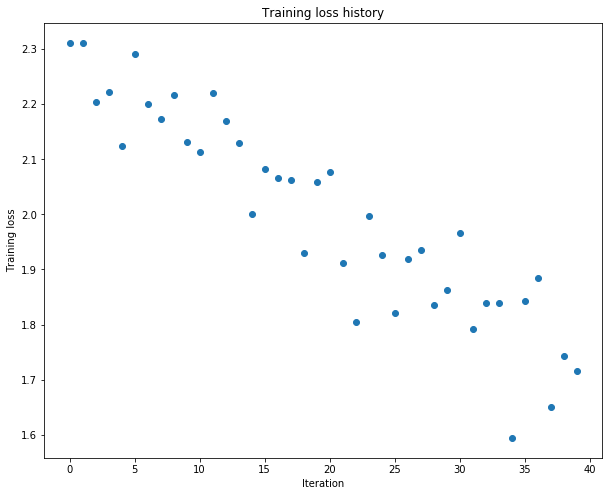
发现loss下降较慢,判断学习率太小了
将learning_rate 设置为 1e-2
(Iteration 1 / 40) loss: 2.330135
(Epoch 0 / 20) train acc: 0.260000; val_acc: 0.097000
(Epoch 1 / 20) train acc: 0.280000; val_acc: 0.109000
(Epoch 2 / 20) train acc: 0.280000; val_acc: 0.129000
(Epoch 3 / 20) train acc: 0.580000; val_acc: 0.146000
(Epoch 4 / 20) train acc: 0.640000; val_acc: 0.133000
(Epoch 5 / 20) train acc: 0.620000; val_acc: 0.176000
(Iteration 11 / 40) loss: 1.567106
(Epoch 6 / 20) train acc: 0.600000; val_acc: 0.176000
(Epoch 7 / 20) train acc: 0.720000; val_acc: 0.122000
(Epoch 8 / 20) train acc: 0.880000; val_acc: 0.162000
(Epoch 9 / 20) train acc: 0.920000; val_acc: 0.160000
(Epoch 10 / 20) train acc: 0.920000; val_acc: 0.187000
(Iteration 21 / 40) loss: 0.496118
(Epoch 11 / 20) train acc: 0.980000; val_acc: 0.175000
(Epoch 12 / 20) train acc: 0.920000; val_acc: 0.156000
(Epoch 13 / 20) train acc: 0.960000; val_acc: 0.179000
(Epoch 14 / 20) train acc: 0.980000; val_acc: 0.182000
(Epoch 15 / 20) train acc: 1.000000; val_acc: 0.175000
(Iteration 31 / 40) loss: 0.076210
(Epoch 16 / 20) train acc: 1.000000; val_acc: 0.192000
(Epoch 17 / 20) train acc: 1.000000; val_acc: 0.180000
(Epoch 18 / 20) train acc: 1.000000; val_acc: 0.173000
(Epoch 19 / 20) train acc: 1.000000; val_acc: 0.178000
(Epoch 20 / 20) train acc: 1.000000; val_acc: 0.175000
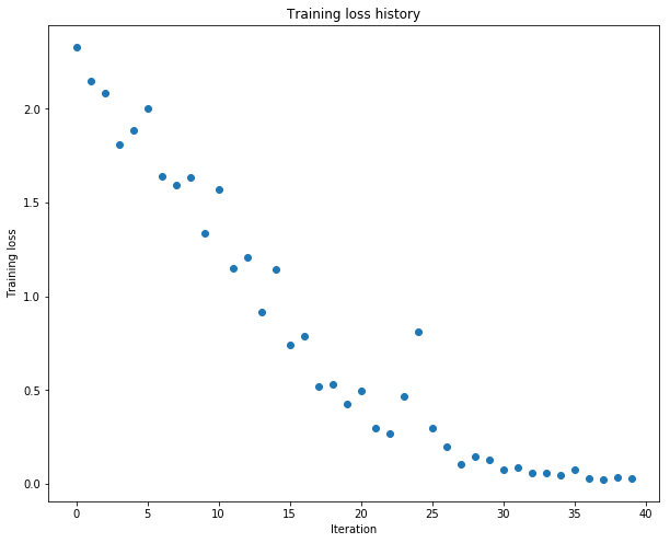
成功的overfit,达到100%的准确率。
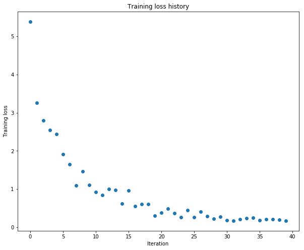
接着测试一个5层网络来overfit50张照片。
使用初始参数:
(Iteration 1 / 40) loss: 2.302585
(Epoch 0 / 20) train acc: 0.160000; val_acc: 0.112000
(Epoch 1 / 20) train acc: 0.100000; val_acc: 0.107000
(Epoch 2 / 20) train acc: 0.100000; val_acc: 0.107000
(Epoch 3 / 20) train acc: 0.120000; val_acc: 0.105000
(Epoch 4 / 20) train acc: 0.160000; val_acc: 0.112000
(Epoch 5 / 20) train acc: 0.160000; val_acc: 0.112000
(Iteration 11 / 40) loss: 2.302211
(Epoch 6 / 20) train acc: 0.160000; val_acc: 0.112000
(Epoch 7 / 20) train acc: 0.160000; val_acc: 0.112000
(Epoch 8 / 20) train acc: 0.160000; val_acc: 0.112000
(Epoch 9 / 20) train acc: 0.160000; val_acc: 0.079000
(Epoch 10 / 20) train acc: 0.160000; val_acc: 0.112000
(Iteration 21 / 40) loss: 2.301766
(Epoch 11 / 20) train acc: 0.160000; val_acc: 0.112000
(Epoch 12 / 20) train acc: 0.160000; val_acc: 0.079000
(Epoch 13 / 20) train acc: 0.160000; val_acc: 0.079000
(Epoch 14 / 20) train acc: 0.160000; val_acc: 0.079000
(Epoch 15 / 20) train acc: 0.160000; val_acc: 0.079000
(Iteration 31 / 40) loss: 2.302234
(Epoch 16 / 20) train acc: 0.160000; val_acc: 0.079000
(Epoch 17 / 20) train acc: 0.160000; val_acc: 0.079000
(Epoch 18 / 20) train acc: 0.160000; val_acc: 0.112000
(Epoch 19 / 20) train acc: 0.160000; val_acc: 0.112000
(Epoch 20 / 20) train acc: 0.160000; val_acc: 0.079000

调整weight_scale = 5e-2之后:
(Iteration 1 / 40) loss: 3.445131
(Epoch 0 / 20) train acc: 0.160000; val_acc: 0.099000
(Epoch 1 / 20) train acc: 0.200000; val_acc: 0.101000
(Epoch 2 / 20) train acc: 0.380000; val_acc: 0.112000
(Epoch 3 / 20) train acc: 0.500000; val_acc: 0.127000
(Epoch 4 / 20) train acc: 0.600000; val_acc: 0.144000
(Epoch 5 / 20) train acc: 0.700000; val_acc: 0.127000
(Iteration 11 / 40) loss: 1.105333
(Epoch 6 / 20) train acc: 0.700000; val_acc: 0.137000
(Epoch 7 / 20) train acc: 0.800000; val_acc: 0.137000
(Epoch 8 / 20) train acc: 0.860000; val_acc: 0.137000
(Epoch 9 / 20) train acc: 0.860000; val_acc: 0.132000
(Epoch 10 / 20) train acc: 0.900000; val_acc: 0.130000
(Iteration 21 / 40) loss: 0.608579
(Epoch 11 / 20) train acc: 0.940000; val_acc: 0.131000
(Epoch 12 / 20) train acc: 0.980000; val_acc: 0.122000
(Epoch 13 / 20) train acc: 0.980000; val_acc: 0.123000
(Epoch 14 / 20) train acc: 0.960000; val_acc: 0.130000
(Epoch 15 / 20) train acc: 0.980000; val_acc: 0.132000
(Iteration 31 / 40) loss: 0.437144
(Epoch 16 / 20) train acc: 0.980000; val_acc: 0.125000
(Epoch 17 / 20) train acc: 0.980000; val_acc: 0.123000
(Epoch 18 / 20) train acc: 0.980000; val_acc: 0.128000
(Epoch 19 / 20) train acc: 1.000000; val_acc: 0.129000
(Epoch 20 / 20) train acc: 1.000000; val_acc: 0.120000
SGD+monentum
def sgd_momentum(w, dw, config=None):
    """
    Performs stochastic gradient descent with momentum.

    config format:
    - learning_rate: Scalar learning rate.
    - momentum: Scalar between 0 and 1 giving the momentum value.
      Setting momentum = 0 reduces to sgd.
    - velocity: A numpy array of the same shape as w and dw used to store a
      moving average of the gradients.
    """
    if config is None: config = {}
    config.setdefault('learning_rate', 1e-2)
    config.setdefault('momentum', 0.9)
    v = config.get('velocity', np.zeros_like(w))

    next_w = None
    ###########################################################################
    # TODO: Implement the momentum update formula. Store the updated value in #
    # the next_w variable. You should also use and update the velocity v.     #
    ###########################################################################
    v = config['momentum'] * v - config['learning_rate'] * dw
    next_w = w + v
    ###########################################################################
    #                             END OF YOUR CODE                            #
    ###########################################################################
    config['velocity'] = v

    return next_w, config
next_w error: 8.882347033505819e-09
velocity error: 4.269287743278663e-09
SGD和SGD with momentum的比较
running with sgd
(Iteration 1 / 200) loss: 2.507323
(Epoch 0 / 5) train acc: 0.102000; val_acc: 0.092000
(Iteration 11 / 200) loss: 2.208203
(Iteration 21 / 200) loss: 2.210458
(Iteration 31 / 200) loss: 2.118780
(Epoch 1 / 5) train acc: 0.251000; val_acc: 0.225000
(Iteration 41 / 200) loss: 2.059379
(Iteration 51 / 200) loss: 2.031150
(Iteration 61 / 200) loss: 1.991460
(Iteration 71 / 200) loss: 1.889502
(Epoch 2 / 5) train acc: 0.311000; val_acc: 0.286000
(Iteration 81 / 200) loss: 1.884040
(Iteration 91 / 200) loss: 1.884515
(Iteration 101 / 200) loss: 1.923375
(Iteration 111 / 200) loss: 1.737657
(Epoch 3 / 5) train acc: 0.343000; val_acc: 0.309000
(Iteration 121 / 200) loss: 1.689422
(Iteration 131 / 200) loss: 1.709433
(Iteration 141 / 200) loss: 1.799477
(Iteration 151 / 200) loss: 1.809359
(Epoch 4 / 5) train acc: 0.415000; val_acc: 0.336000
(Iteration 161 / 200) loss: 1.599980
(Iteration 171 / 200) loss: 1.732295
(Iteration 181 / 200) loss: 1.740551
(Iteration 191 / 200) loss: 1.634729
(Epoch 5 / 5) train acc: 0.403000; val_acc: 0.354000
running with sgd_momentum
(Iteration 1 / 200) loss: 2.677090
(Epoch 0 / 5) train acc: 0.100000; val_acc: 0.092000
(Iteration 11 / 200) loss: 2.118401
(Iteration 21 / 200) loss: 2.122486
(Iteration 31 / 200) loss: 1.851282
(Epoch 1 / 5) train acc: 0.326000; val_acc: 0.287000
(Iteration 41 / 200) loss: 1.852963
(Iteration 51 / 200) loss: 1.920911
(Iteration 61 / 200) loss: 1.798175
(Iteration 71 / 200) loss: 1.714354
(Epoch 2 / 5) train acc: 0.386000; val_acc: 0.303000
(Iteration 81 / 200) loss: 1.882377
(Iteration 91 / 200) loss: 1.572796
(Iteration 101 / 200) loss: 1.854254
(Iteration 111 / 200) loss: 1.500233
(Epoch 3 / 5) train acc: 0.480000; val_acc: 0.348000
(Iteration 121 / 200) loss: 1.516018
(Iteration 131 / 200) loss: 1.592710
(Iteration 141 / 200) loss: 1.524653
(Iteration 151 / 200) loss: 1.340690
(Epoch 4 / 5) train acc: 0.478000; val_acc: 0.321000
(Iteration 161 / 200) loss: 1.297253
(Iteration 171 / 200) loss: 1.460615
(Iteration 181 / 200) loss: 1.113488
(Iteration 191 / 200) loss: 1.550920
(Epoch 5 / 5) train acc: 0.512000; val_acc: 0.327000
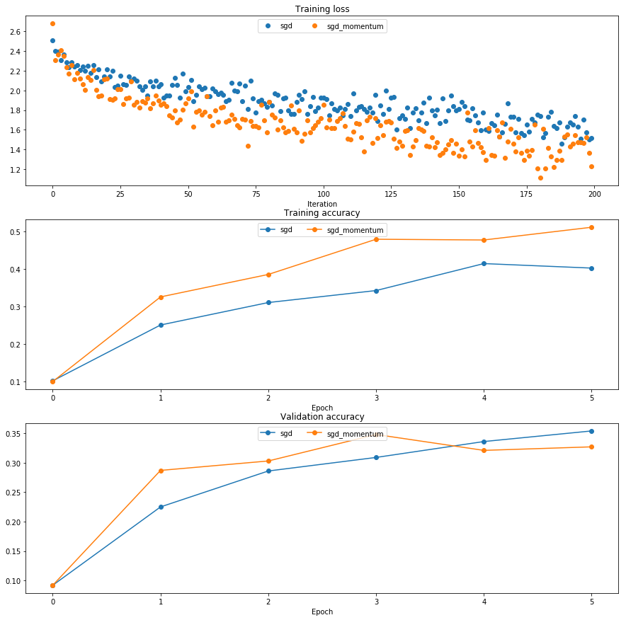
发现SGD+momentum的loss下降更快
测试RMSprop
def rmsprop(w, dw, config=None):
    """
    Uses the RMSProp update rule, which uses a moving average of squared
    gradient values to set adaptive per-parameter learning rates.

    config format:
    - learning_rate: Scalar learning rate.
    - decay_rate: Scalar between 0 and 1 giving the decay rate for the squared
      gradient cache.
    - epsilon: Small scalar used for smoothing to avoid dividing by zero.
    - cache: Moving average of second moments of gradients.
    """
    if config is None: config = {}
    config.setdefault('learning_rate', 1e-2)
    config.setdefault('decay_rate', 0.99)
    config.setdefault('epsilon', 1e-8)
    config.setdefault('cache', np.zeros_like(w))

    next_w = None
    ###########################################################################
    # TODO: Implement the RMSprop update formula, storing the next value of w #
    # in the next_w variable. Don't forget to update cache value stored in    #
    # config['cache'].                                                        #
    ###########################################################################
    config['cache'] = config['cache'] * config['decay_rate'] + (1 - config['decay_rate']) *dw * dw #让累积的平方梯度按照一定比率下降
    next_w = w - config['learning_rate'] * dw / np.sqrt(config['cache'] + config['epsilon'])
    ###########################################################################
    #                             END OF YOUR CODE                            #
    ###########################################################################

    return next_w, config
next_w error: 9.502645229894295e-08
cache error: 2.6477955807156126e-09
测试adam:
def adam(w, dw, config=None):
    """
    Uses the Adam update rule, which incorporates moving averages of both the
    gradient and its square and a bias correction term.

    config format:
    - learning_rate: Scalar learning rate.
    - beta1: Decay rate for moving average of first moment of gradient.
    - beta2: Decay rate for moving average of second moment of gradient.
    - epsilon: Small scalar used for smoothing to avoid dividing by zero.
    - m: Moving average of gradient.
    - v: Moving average of squared gradient.
    - t: Iteration number.
    """
    if config is None: config = {}
    config.setdefault('learning_rate', 1e-3)
    config.setdefault('beta1', 0.9)
    config.setdefault('beta2', 0.999)
    config.setdefault('epsilon', 1e-8)
    config.setdefault('m', np.zeros_like(w))
    config.setdefault('v', np.zeros_like(w))
    config.setdefault('t', 0)

    next_w = None
    ###########################################################################
    # TODO: Implement the Adam update formula, storing the next value of w in #
    # the next_w variable. Don't forget to update the m, v, and t variables   #
    # stored in config.                                                       #
    #                                                                         #
    # NOTE: In order to match the reference output, please modify t _before_  #
    # using it in any calculations.                                           #
    ###########################################################################
    m = config['m'] * config['beta1'] + (1 - config['beta1']) * dw
    v = config['v'] * config['beta2'] + (1 - config['beta2']) * dw * dw
    config['t'] = 1
    mb = m / (1 - config['beta1'] ** config['t'])
    vb = v / (1 - config['beta2'] ** config['t'])
    next_w = w - config['learning_rate'] * mb / (np.sqrt(vb) + config['epsilon']) #综合了momentum和RMSProp
    config['m'] = m
    config['v'] = v
    ###########################################################################
    #                             END OF YOUR CODE                            #
    ###########################################################################

    return next_w, config
next_w error: 0.032064274004801614
v error: 4.208314038113071e-09
m error: 4.214963193114416e-09
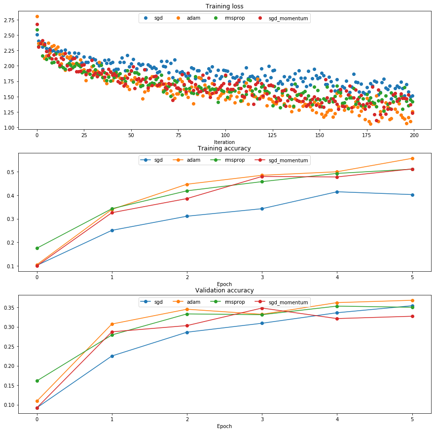
三种优化算法在训练中的比较:
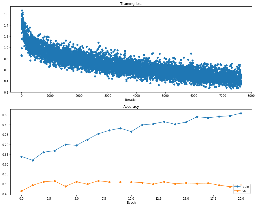
训练一个网络!一个3层的全连接网络,有dropout和batchnorm。
best_model = None
################################################################################
# TODO: Train the best FullyConnectedNet that you can on CIFAR-10. You might #
# find batch/layer normalization and dropout useful. Store your best model in #
# the best_model variable. #
################################################################################
dropout = 0.25
weight_scale = 2e-2
lr = 1e-3
hidden_dims = [1024,1024,1024]
best_model = FullyConnectedNet(hidden_dims = hidden_dims,num_classes = 10,
weight_scale = weight_scale,normalization='batchnorm',
dropout = dropout)
solver = Solver(model,data,num_epochs = 10,batch_size = 128,print_every = 100,
update_rule = 'adam',verbose = True,optim_config = {'learning_rate': lr})
solver.train()
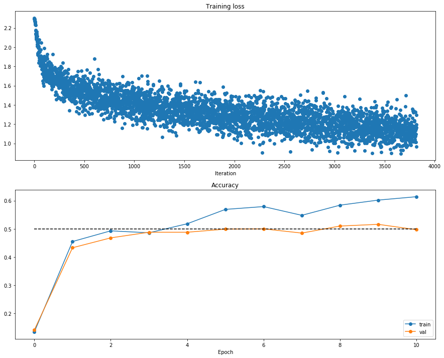
plt.subplot(2, 1, 1)
plt.title('Training loss')
plt.plot(solver.loss_history, 'o')
plt.xlabel('Iteration')
plt.subplot(2, 1, 2)
plt.title('Accuracy')
plt.plot(solver.train_acc_history, '-o', label='train')
plt.plot(solver.val_acc_history, '-o', label='val')
plt.plot([0.5] * len(solver.val_acc_history), 'k--')
plt.xlabel('Epoch')
plt.legend(loc='lower right')
plt.gcf().set_size_inches(15, 12)
plt.show()
################################################################################
# END OF YOUR CODE #
################################################################################
Iteration = 49000//128*20 = 7640
(Iteration 1 / 7640) loss: 0.859818
(Epoch 0 / 20) train acc: 0.639000; val_acc: 0.464000
(Iteration 101 / 7640) loss: 1.252969
(Iteration 201 / 7640) loss: 1.065346
(Iteration 301 / 7640) loss: 0.863103
(Epoch 1 / 20) train acc: 0.620000; val_acc: 0.493000
(Iteration 401 / 7640) loss: 1.136908
(Iteration 501 / 7640) loss: 0.960427
(Iteration 601 / 7640) loss: 0.967821
(Iteration 701 / 7640) loss: 0.889575
(Epoch 2 / 20) train acc: 0.661000; val_acc: 0.511000
(Iteration 801 / 7640) loss: 0.842937
(Iteration 901 / 7640) loss: 0.948296
(Iteration 1001 / 7640) loss: 1.020871
(Iteration 1101 / 7640) loss: 1.042730
(Epoch 3 / 20) train acc: 0.668000; val_acc: 0.515000
(Iteration 1201 / 7640) loss: 0.848133
(Iteration 1301 / 7640) loss: 0.824475
(Iteration 1401 / 7640) loss: 0.901598
(Iteration 1501 / 7640) loss: 0.835679
(Epoch 4 / 20) train acc: 0.700000; val_acc: 0.488000
(Iteration 1601 / 7640) loss: 0.692962
(Iteration 1701 / 7640) loss: 0.883259
(Iteration 1801 / 7640) loss: 0.751739
(Iteration 1901 / 7640) loss: 0.834902
(Epoch 5 / 20) train acc: 0.695000; val_acc: 0.511000
(Iteration 2001 / 7640) loss: 0.840407
(Iteration 2101 / 7640) loss: 0.736310
(Iteration 2201 / 7640) loss: 0.736240
(Epoch 6 / 20) train acc: 0.725000; val_acc: 0.499000
(Iteration 2301 / 7640) loss: 0.862586
(Iteration 2401 / 7640) loss: 0.927217
(Iteration 2501 / 7640) loss: 0.755900
(Iteration 2601 / 7640) loss: 0.585035
(Epoch 7 / 20) train acc: 0.754000; val_acc: 0.516000
(Iteration 2701 / 7640) loss: 0.620836
(Iteration 2801 / 7640) loss: 0.659957
(Iteration 2901 / 7640) loss: 0.599932
(Iteration 3001 / 7640) loss: 0.609260
(Epoch 8 / 20) train acc: 0.771000; val_acc: 0.510000
(Iteration 3101 / 7640) loss: 0.783430
(Iteration 3201 / 7640) loss: 0.566388
(Iteration 3301 / 7640) loss: 0.604077
(Iteration 3401 / 7640) loss: 0.515016
(Epoch 9 / 20) train acc: 0.782000; val_acc: 0.510000
(Iteration 3501 / 7640) loss: 0.745964
(Iteration 3601 / 7640) loss: 0.862417
(Iteration 3701 / 7640) loss: 0.528430
(Iteration 3801 / 7640) loss: 0.662338
(Epoch 10 / 20) train acc: 0.765000; val_acc: 0.510000
(Iteration 3901 / 7640) loss: 0.639553
(Iteration 4001 / 7640) loss: 0.685763
(Iteration 4101 / 7640) loss: 0.748629
(Iteration 4201 / 7640) loss: 0.620021
(Epoch 11 / 20) train acc: 0.799000; val_acc: 0.507000
(Iteration 4301 / 7640) loss: 0.646508
(Iteration 4401 / 7640) loss: 0.597432
(Iteration 4501 / 7640) loss: 0.666086
(Epoch 12 / 20) train acc: 0.804000; val_acc: 0.499000
(Iteration 4601 / 7640) loss: 0.619035
(Iteration 4701 / 7640) loss: 0.685448
(Iteration 4801 / 7640) loss: 0.786623
(Iteration 4901 / 7640) loss: 0.566107
(Epoch 13 / 20) train acc: 0.815000; val_acc: 0.511000
(Iteration 5001 / 7640) loss: 0.551514
(Iteration 5101 / 7640) loss: 0.597256
(Iteration 5201 / 7640) loss: 0.643402
(Iteration 5301 / 7640) loss: 0.524270
(Epoch 14 / 20) train acc: 0.802000; val_acc: 0.501000
(Iteration 5401 / 7640) loss: 0.569950
(Iteration 5501 / 7640) loss: 0.522419
(Iteration 5601 / 7640) loss: 0.644923
(Iteration 5701 / 7640) loss: 0.513421
(Epoch 15 / 20) train acc: 0.813000; val_acc: 0.505000
(Iteration 5801 / 7640) loss: 0.489016
(Iteration 5901 / 7640) loss: 0.408196
(Iteration 6001 / 7640) loss: 0.382298
(Iteration 6101 / 7640) loss: 0.540364
(Epoch 16 / 20) train acc: 0.840000; val_acc: 0.503000
(Iteration 6201 / 7640) loss: 0.418339
(Iteration 6301 / 7640) loss: 0.578868
(Iteration 6401 / 7640) loss: 0.412187
(Epoch 17 / 20) train acc: 0.835000; val_acc: 0.504000
(Iteration 6501 / 7640) loss: 0.541283
(Iteration 6601 / 7640) loss: 0.462409
(Iteration 6701 / 7640) loss: 0.509253
(Iteration 6801 / 7640) loss: 0.505827
(Epoch 18 / 20) train acc: 0.841000; val_acc: 0.494000
(Iteration 6901 / 7640) loss: 0.476122
(Iteration 7001 / 7640) loss: 0.528972
(Iteration 7101 / 7640) loss: 0.533508
(Iteration 7201 / 7640) loss: 0.598713
(Epoch 19 / 20) train acc: 0.845000; val_acc: 0.486000
(Iteration 7301 / 7640) loss: 0.473737
(Iteration 7401 / 7640) loss: 0.443160
(Iteration 7501 / 7640) loss: 0.332309
(Iteration 7601 / 7640) loss: 0.300785
(Epoch 20 / 20) train acc: 0.858000; val_acc: 0.497000
参考:https://blog.csdn.net/BigDataDigest/article/details/79286510